
Are certain individuals more predisposed to being driven by promotions and offers? That is, can we identify certain individuals who will engage (ie. spend more) with our business solely based on offers, such as discounts, that are made available to them? In the case of Starbucks, my analysis has found little to no correlation between the total spending from customers and the kinds or amounts of offers made available to them. This is not to say that offers and promotions are not effective - in fact, I suggest that future works focus on how to maximize the effectiveness of our offers. However, when we look at regular Starbucks mobile app users and their overall engagement with Starbucks, I see little correlation in the types of offers being made and the total amount they spend at Starbucks. As a result of this analysis, I suggest that future analytics efforts focus on the promotions themselves and how to make them effective, as opposed to identifying specific demographics that will respond strongly to promotions.
Starbucks has provided students enrolled in Udacity's data science nanodegree with simulated data for users of the Starbucks mobile app. In this dataset, 17000 users have been simulated, and we have been provided with demographic information for each of these simulated users. Additionally, information on the different types of promotions which have been offered to these users is provided.
This simulated data takes place over a 30 day period, during which 167,581 offers were made to these customers, and 138,953 purchases were made. At a high level, I have been asked to identify effective uses of promotions in the future.
There are a wide variety of questions which could be asked of these data. Are buy-one-get-one (bogo) offers more effective at driving engagement than discounts? Do shorter durations of offer availability drive more frequent engagement? Are certain demographics more likely to respond to certain types of promotions?
In this analysis, I have chosen to focus on overall customer spending and its relation to promotions. Specifically, I woud like to identify the type of relationship, or lack thereof, between the offers being made to customers and their relative spending at Starbucks. In other words, with all else being equal, do Starbucks app users (referred to as users hereon) who receive more offers or specific kinds of offers spend significantly more than average? Included in this question is the efficacy of certain promotion types or communication channels. For instance, are do discounts drive more spending from users than bogo offers? Is email more effective at driving spending than social media?
I have selected "overall spend" (spend from hereon) as my primary metric for efficacy of promotions. Specifically, I will consider the total spending per-customer over the 30 day period of this experiment as my primary metric. If I have a group of demographically similar people, is their spend correlated to the types and amounts of offers they received during this period?
There are several other variables that coud be used as metrics, such as "was this particular offer viewed and/or completed," and "number of visits to starbucks during this time period." However, while these may be useful (they almost certainly are!) for evaluating the efficacy of certain promotions, Starbucks is ultimately not in the business of making effective promotions. Starbucks will want to maximize revenue, which is related to maximizing spending per customer.
An interesting wrinkle in this analysis is the goal of maximizing revenue, and not necessarily spending-per-customer. An extreme implication of this is if we have "superusers," users who spend so much at Starbucks that they make up a disproportionately large amount of the profit base. It will be a much more effective user of our time to increase spending from our primary profit base than to try and increase every individuals' spending. As such, we will try to focus our analysis on demographics that could potentially have the greatest impact on overall profit.
Three tables of data have been provided by Starbucks for this analysis:
It is useful to understand the ranges for some of these categories.
profile["gender"].value_counts(dropna=False)

===== GENDER ======
M       8484
F       6129
None    2175
O        212
Slightly more men have been simulated in this study - I will assume that this is representative of the actual users in the true Starbucks app. Additionally, exploring other fields reveals that users who replied "None" also lack any identifying information for age or income. As I am interesting in comparing like users for the efficacy of promos, we will probably exclude these users.
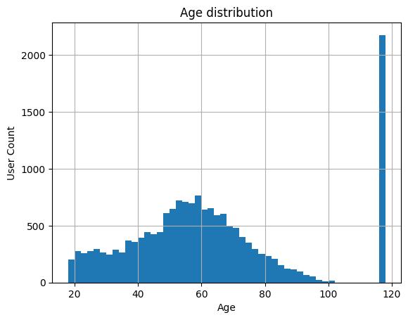
Ages are normally distributed. It looks like the minimum allowed user age is 18 - it is possible that there is a bump here because users either user 18 as a default, or underage users just say they are 18. This is not a major issue, as the data looks basically normal. The major spike at 118 is a default value, and corresponds to "None" entries on gender - we will ignore these.
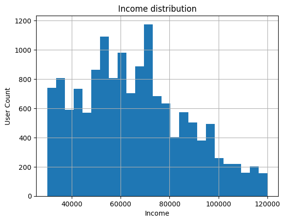
>>> profile.income.describe()
===== INCOME ======
count     14825.000000
mean      65404.991568
std       21598.299410
min       30000.000000
25%       49000.000000
50%       64000.000000
75%       80000.000000
max      120000.000000
Data skews to the right, and this generally looks as expected.
"became_member_on" is a trickier field - it would be more useful if this was numeric and it described the length of a users's membership, in days. We will create this value, and call it "tenure".
profile["joindate"] = pd.to_datetime(profile["became_member_on"],format="%Y%m%d")
profile["tenure"] = (profile["joindate"] - profile["joindate"].min()).dt.days
>>> profile.tenure.describe()
count    17000.000000
mean      1305.550118
std        411.223904
min          0.000000
25%       1032.000000
50%       1465.000000
75%       1615.000000
max       1823.000000
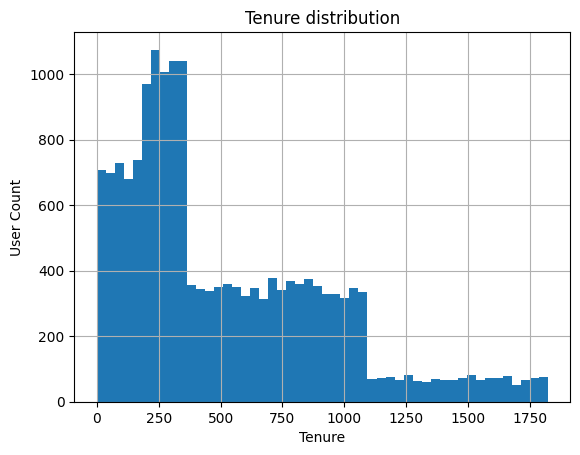
This is a very strange looking distribution to me. There must have been major pushes for membership at certain points in time, causing new users to be introduced.
>>> print(transcript.event.value_counts(dropna=False))
transaction        138953
offer received      76277
offer viewed        57725
offer completed     33579
Not quite half of our events are transactions, and we see descending values of offers received, viewed, and completed. This is not surprising.
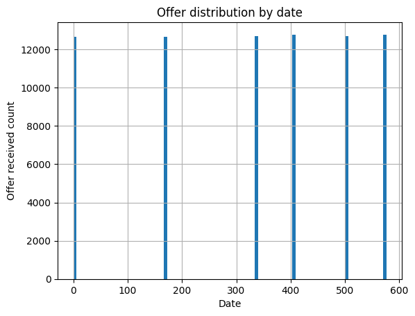
During the experimental period, there were fixed days on which offers would go out to customers. This is pretty useful for comparing the efficacy of one offer versus another.
The transcript is not easy to read in its current state. If I join the portfolio data to it, I can explore the offer types much more easily.
df = transcript.merge(profile,how='left',left_on='person',right_on='id')
df = df[[
    "person",
    "event",
    "value",
    "time",
    "gender",
    "age",
    "income",
    "tenure"
]]

df["amount"] = df.value.apply(lambda x: x.get("amount",0))
df["offerid"] = df.value.apply(lambda x: x.get("offer id",x.get("offer_id",0)))

df = df.merge(portfolio, how='left', left_on="offerid", right_on="id")

df = df[[
    "person",
    "event",
    # "value",
    "time",
    "gender",
    "age",
    "income",
    "tenure",
    "amount",
    'offername',
    'channels',
    'reward',
    'difficulty',
    'duration',
    'offer_type',
    'mobile',
    'web',
    'social',
    'email',
]]

df.time = df.time/24.0

df.head()
| person | event | time | gender | age | income | tenure | amount | offername | channels | reward | difficulty | duration | offer_type | mobile | web | social | ||
|---|---|---|---|---|---|---|---|---|---|---|---|---|---|---|---|---|---|---|
| 0 | 78afa995795e4d85b5d9ceeca43f5fef | offer received | 0 | F | 75 | 100000 | 443 | 0 | bogo_7_5_5 | ['web', 'email', 'mobile'] | 5 | 5 | 7 | bogo | 1 | 1 | 0 | 1 |
| 1 | a03223e636434f42ac4c3df47e8bac43 | offer received | 0 | 118 | nan | 356 | 0 | discount_10_20_5 | ['web', 'email'] | 5 | 20 | 10 | discount | 0 | 1 | 0 | 1 | |
| 2 | e2127556f4f64592b11af22de27a7932 | offer received | 0 | M | 68 | 70000 | 91 | 0 | discount_7_10_2 | ['web', 'email', 'mobile'] | 2 | 10 | 7 | discount | 1 | 1 | 0 | 1 |
| 3 | 8ec6ce2a7e7949b1bf142def7d0e0586 | offer received | 0 | 118 | nan | 304 | 0 | discount_10_10_2 | ['web', 'email', 'mobile', 'social'] | 2 | 10 | 10 | discount | 1 | 1 | 1 | 1 | |
| 4 | 68617ca6246f4fbc85e91a2a49552598 | offer received | 0 | 118 | nan | 297 | 0 | bogo_5_10_10 | ['web', 'email', 'mobile', 'social'] | 10 | 10 | 5 | bogo | 1 | 1 | 1 | 1 |
Now that I have the channel data one-hot encoded, as well as adding in offer information, it is much easier to understand the transcript data.
As stated above, I am interested in understanding how to maximize profit from the most profitable base using promotions. This means I will summarize the data on a per-user basis, and examine how certain factors affect profitability.
I will create a detailed "person" table, and then explore it visually.
person_g = df.groupby([
    "person",
    "gender",
    "age",
    "income",
    "tenure"
])

person_spend = person_g.amount.sum()
person_mobile = person_g.mobile.sum()
person_web = person_g.web.sum()
person_social = person_g.social.sum()
person_email = person_g.email.sum()

person_g_offersonly = df[df.event == "offer received"].groupby([
    "person",
    "gender",
    "age",
    "income",
    "tenure"
])

person_offers_total = person_g_offersonly.offername.count()

person_offers = df[df.event == "offer received"].pivot_table(index=[
    "person",
    "gender",
    "age",
    "income",
    "tenure"
], columns='offername', aggfunc='size', fill_value=0)

person_offers_type = df[df.event == "offer received"].pivot_table(index=[
    "person",
    "gender",
    "age",
    "income",
    "tenure"
], columns='offer_type', aggfunc='size', fill_value=0)

person_events = df.pivot_table(index=[
    "person",
    "gender",
    "age",
    "income",
    "tenure"
], columns='event', aggfunc='size', fill_value=0)

for col in person_events:
    person_offers[col] = person_events[col]

for col in person_offers_type:
    person_offers[col] = person_offers_type[col]

person_offers["spend"] = person_spend
person_offers["totaloffers"] = person_offers_total
person_offers["spendpertransaction"] = person_offers["spend"] / person_offers["transaction"]

person_offers["mobile"] = person_mobile
person_offers["web"] = person_web
person_offers["social"] = person_social
person_offers["email"] = person_email

# person_offers

df_p = person_offers.reset_index()
df_p.head()
| person | gender | age | income | tenure | bogo_5_10_10 | bogo_5_5_5 | bogo_7_10_10 | bogo_7_5_5 | discount_10_10_2 | discount_10_20_5 | discount_7_10_2 | discount_7_7_3 | informational_3_0_0 | informational_4_0_0 | offer completed | offer received | offer viewed | transaction | bogo | discount | informational | spend | totaloffers | spendpertransaction | mobile | web | social | age_bin | bin | spend_bin | ||
|---|---|---|---|---|---|---|---|---|---|---|---|---|---|---|---|---|---|---|---|---|---|---|---|---|---|---|---|---|---|---|---|---|
| 0 | 0009655768c64bdeb2e877511632db8f | M | 33 | 72000 | 461 | 0 | 1 | 0 | 0 | 1 | 0 | 1 | 0 | 1 | 1 | 3 | 5 | 4 | 8 | 1 | 2 | 2 | 127.6 | 5 | 15.95 | 12 | 10 | 8 | 12 | 30 | 12 | 125 |
| 1 | 0011e0d4e6b944f998e987f904e8c1e5 | O | 40 | 57000 | 198 | 0 | 0 | 0 | 1 | 0 | 1 | 0 | 1 | 1 | 1 | 3 | 5 | 5 | 5 | 1 | 2 | 2 | 79.46 | 5 | 15.892 | 10 | 11 | 5 | 13 | 40 | 13 | 75 |
| 2 | 0020c2b971eb4e9188eac86d93036a77 | F | 59 | 90000 | 874 | 1 | 0 | 1 | 0 | 2 | 0 | 0 | 0 | 1 | 0 | 3 | 5 | 3 | 8 | 2 | 2 | 1 | 196.86 | 5 | 24.6075 | 11 | 8 | 11 | 11 | 55 | 11 | 195 |
| 3 | 0020ccbbb6d84e358d3414a3ff76cffd | F | 24 | 60000 | 622 | 0 | 1 | 0 | 1 | 0 | 0 | 0 | 1 | 1 | 0 | 3 | 4 | 4 | 12 | 2 | 1 | 1 | 154.05 | 4 | 12.8375 | 11 | 9 | 8 | 11 | 20 | 11 | 150 |
| 4 | 003d66b6608740288d6cc97a6903f4f0 | F | 26 | 73000 | 400 | 0 | 0 | 0 | 0 | 2 | 1 | 0 | 0 | 1 | 1 | 3 | 5 | 4 | 18 | 0 | 3 | 2 | 48.34 | 5 | 2.68556 | 10 | 10 | 8 | 12 | 25 | 12 | 45 |
This has created an extensive customer profile table. Some key values in here include the amount of offers received per customer, the total spend per customer, the spend-per-transaction, total transaction count, and the counts of communication channels used.
Already, we see a potential weakness in this analysis - we will not be looking at duration, difficulty, and rewards of offers. However, this is not the goal of our analysis - we want to understand if there are specific groups of customers who are, overall, more interested in promotions than others, and if this drives profits.
Since we are interested in maximizing profits, I will explore spending and its relationships a little bit:
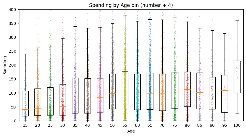
The median spending of users almost doubles as their age goes from 18-19 to 55-60. Interestingly, all of these plots have very long upward tails, which may indicate that our profit base may be with higher-spenders.
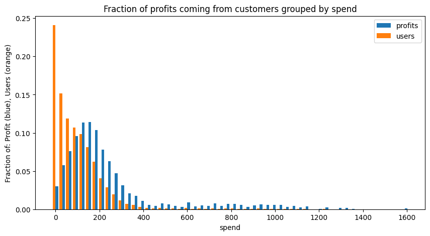
This is an interesting plot. The blue bars represent "fraction of total profits". The X-axis is the total spending by a customer. The orange bars represent the fraction of users who actually spend that amount. What this means is that, while our customers have a right-skewing distribution (ie there are many users who only spend a small amount), our profits are centered around users who spend $150 to $200 a month. Any analysis we want to do should focus on maximizing engagement from this group.
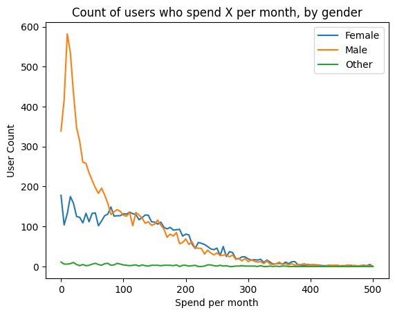
Interestingly, we notice a distinct difference in spending between men and women. Men have a much higher number of "low spenders", but otherwise they have similar looking profiles. It may be that casual starbucks users who are male are more likely to become app users, but otherwise superusers who are male or female behave similarly.
Later in our modeling, we will exclude low spenders, since these two plots show that: 1. Only a small amount of our profits come from low spenders 2. We have reason to believe that these users behave differently from the rest of the user population, and their behavior may alter our modeling.
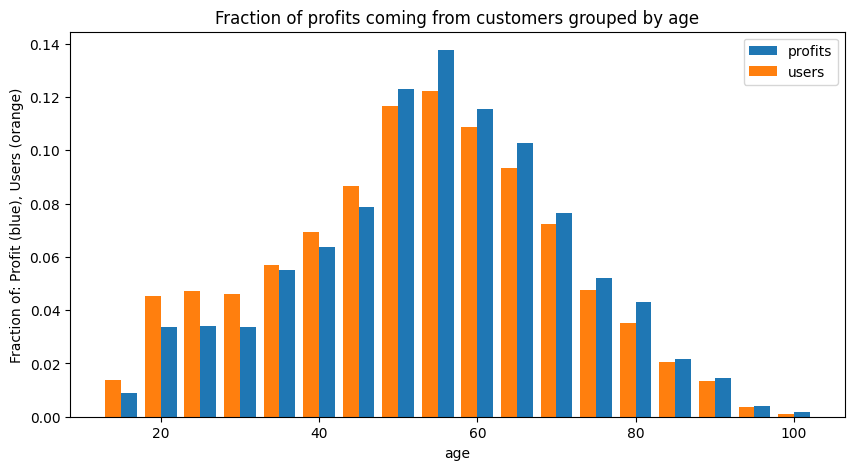
Interstingly, our profit base appears to be fairly well-distributed among our ages. This agrees with our spending-by-age plot above - younger people spend a little less than older users, and we see here that our profit base skews to older users, but not by much.
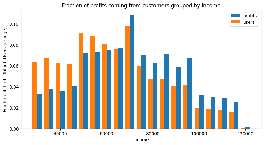
Similar to our age profiling, we see some skewing of our profit base by user income, but not by much.
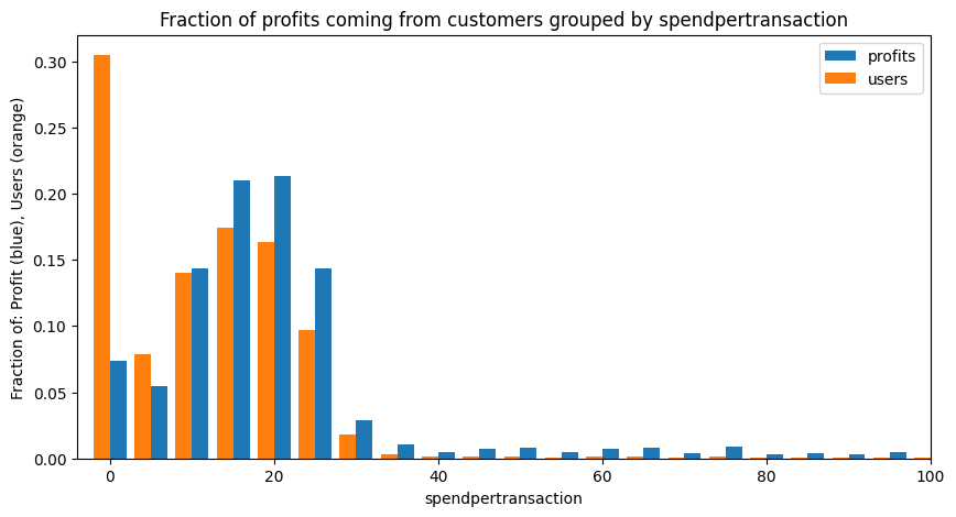
Spend-per-transaction is very important for our profit base. Users who spend $0-$4 per transaction make up nearly 30% of the user base, but account for only about 7% of profits. This further indicates that we will want to focus on driving engagement from our most profitable users.
I would now like to start understanding how the offers being made to the customers work in driving profits.
def show_corr(df):
    df_p_corr = df[[
        "age",
        "income",
        "tenure",
        'offer received',
        "offer viewed",
        "offer completed",
        "transaction",
        "spend",
        "spendpertransaction",
        "mobile",
        "web",
        "social",
        "email",
        "totaloffers"
    ]]

    corr = df_p_corr.corr()
    return corr.style.background_gradient(cmap='coolwarm',vmin=-1,vmax=1)

show_corr(df_p)
| offername | age | income | tenure | offer received | offer viewed | offer completed | transaction | spend | spendpertransaction | mobile | web | social | totaloffers | |
|---|---|---|---|---|---|---|---|---|---|---|---|---|---|---|
| offername | ||||||||||||||
| age | 1.000000 | 0.306949 | 0.012195 | -0.004772 | 0.038346 | 0.114451 | -0.155693 | 0.105963 | 0.201019 | 0.055417 | 0.068625 | 0.024114 | 0.072471 | -0.004772 |
| income | 0.306949 | 1.000000 | 0.025619 | -0.006837 | 0.052495 | 0.257844 | -0.266195 | 0.314995 | 0.492497 | 0.118431 | 0.134167 | 0.063999 | 0.150559 | -0.006837 |
| tenure | 0.012195 | 0.025619 | 1.000000 | -0.005587 | 0.018851 | 0.225664 | 0.425925 | 0.166252 | 0.021718 | 0.107398 | 0.105958 | 0.063168 | 0.120668 | -0.005587 |
| offer received | -0.004772 | -0.006837 | -0.005587 | 1.000000 | 0.579838 | 0.333138 | 0.159570 | 0.089759 | 0.000657 | 0.683744 | 0.580987 | 0.479856 | 0.754496 | 1.000000 |
| offer viewed | 0.038346 | 0.052495 | 0.018851 | 0.579838 | 1.000000 | 0.398355 | 0.206257 | 0.203420 | 0.099374 | 0.796823 | 0.602837 | 0.657127 | 0.817161 | 0.579838 |
| offer completed | 0.114451 | 0.257844 | 0.225664 | 0.333138 | 0.398355 | 1.000000 | 0.417161 | 0.537165 | 0.308771 | 0.683116 | 0.713606 | 0.492560 | 0.788620 | 0.333138 |
| transaction | -0.155693 | -0.266195 | 0.425925 | 0.159570 | 0.206257 | 0.417161 | 1.000000 | 0.347370 | -0.127814 | 0.342733 | 0.279849 | 0.311255 | 0.352702 | 0.159570 |
| spend | 0.105963 | 0.314995 | 0.166252 | 0.089759 | 0.203420 | 0.537165 | 0.347370 | 1.000000 | 0.757001 | 0.339404 | 0.315392 | 0.255171 | 0.388506 | 0.089759 |
| spendpertransaction | 0.201019 | 0.492497 | 0.021718 | 0.000657 | 0.099374 | 0.308771 | -0.127814 | 0.757001 | 1.000000 | 0.154899 | 0.163387 | 0.091571 | 0.196797 | 0.000657 |
| mobile | 0.055417 | 0.118431 | 0.107398 | 0.683744 | 0.796823 | 0.683116 | 0.342733 | 0.339404 | 0.154899 | 1.000000 | 0.710980 | 0.754441 | 0.913526 | 0.683744 |
| web | 0.068625 | 0.134167 | 0.105958 | 0.580987 | 0.602837 | 0.713606 | 0.279849 | 0.315392 | 0.163387 | 0.710980 | 1.000000 | 0.424316 | 0.813168 | 0.580987 |
| social | 0.024114 | 0.063999 | 0.063168 | 0.479856 | 0.657127 | 0.492560 | 0.311255 | 0.255171 | 0.091571 | 0.754441 | 0.424316 | 1.000000 | 0.688414 | 0.479856 |
| 0.072471 | 0.150559 | 0.120668 | 0.754496 | 0.817161 | 0.788620 | 0.352702 | 0.388506 | 0.196797 | 0.913526 | 0.813168 | 0.688414 | 1.000000 | 0.754496 | |
| totaloffers | -0.004772 | -0.006837 | -0.005587 | 1.000000 | 0.579838 | 0.333138 | 0.159570 | 0.089759 | 0.000657 | 0.683744 | 0.580987 | 0.479856 | 0.754496 | 1.000000 |
At first glance, we do not see any offer parameters that correlate strongly to spend, transaction, or spendpertransaction. "Offer completed" has a decent correlation to spend, but this value will trigger even if a value was never viewed - both "Offer received" and "Offer viewed" have poor correlations in this regard.
This is a very high-level view of the data. I will now take a more regimented approach to developing a model that could possibly identify if a certain style of engagement drives better profit from a user.
My goal is to develop a model which can fit Starbucks' activities around promotions to overall spend of a customer. Specifically, per customer, we want to see the correlation between: - Inputs: - bogo count received - discount count received - informational count received - total offers received - mobile offers received - web offers received - social offers received - email offers received - Ouput: - total spend during test period.
Optionally, if I see a strong correlation, I will use it to maximize the types of offers we send to customers.
I already know that there are some spending habit differences inherent in age and income. To minimize this, I will look at each users' relative spending to the mean of their demographic.
I can start with our per-person table, which has been used for visualizations above. I also want to remove outliers, so I will only consider users who spend less than $400 a month. Additionally, I saw that users who spend less than $10 per transaction only account for 7% of our profits, so I will focus on our profit base by considersing users whose mean spend-per-transaction is at least $10.
# paired difference modeling:
df_pair = df_p[df_p["spendpertransaction"]>=10][df_p.spend <= 400][[
    "age",
    "income",
    "tenure",
    "bogo",
    "discount",
    "informational",
    "totaloffers",
    "offer viewed",
    "offer completed",
    "mobile",
    "web",
    "social",
    "email",
    "spend",
    "spendpertransaction",
    "transaction"
]]
df_pair["income_bin"] = (df_pair.income // 10000)*10000
df_pair["age_bin"] = (df_pair.age // 10) * 10

# within each group, get the means for spend, transaction, and spendpertransaction. report these back to df_pair. do corr on these.

df_summary = df_pair.groupby(["income_bin","age_bin"])[["spend","transaction","spendpertransaction"]].mean()
df_std = df_pair.groupby(["income_bin","age_bin"])[["spend","transaction","spendpertransaction"]].std()
df_groupsize = df_pair.groupby(["income_bin","age_bin"])["spend"].count()

df_summary["spend_std"] = df_std.spend
df_summary["transaction_std"] = df_std.transaction
df_summary["spendpertransaction_std"] = df_std.spendpertransaction
df_summary["groupsize"] = df_groupsize

df_lookup_bins = df_summary.reset_index()

df_paired_means = df_pair.merge(df_lookup_bins, how='left', left_on=["age_bin","income_bin"], right_on=["age_bin","income_bin"], suffixes = ("","_mean"))
df_paired_means = df_paired_means[[
    "income_bin",
    "age_bin",
    "bogo",
    "discount",
    "informational",
    "totaloffers",
    "offer viewed",
    "offer completed",
    "mobile",
    "web",
    "social",
    "email",
    "spend",
    "spend_mean",
    "spend_std",
    "transaction",
    "transaction_mean",
    "transaction_std",
    "spendpertransaction",
    "spendpertransaction_mean",
    "spendpertransaction_std",
]]
df_paired_means["spend_rel"] = df_paired_means.spend - df_paired_means.spend_mean
df_paired_means["transaction_rel"] = df_paired_means.transaction - df_paired_means.transaction_mean
df_paired_means["spendpertransaction_rel"] = df_paired_means.spendpertransaction - df_paired_means.spendpertransaction_mean
Before modeling this data, it will be useful to look at the correlation matrix for it:
df_pair_corr = df_paired_means[[
    "bogo",
    "discount",
    "informational",
    "totaloffers",
    "offer viewed",
    "offer completed",
    "mobile",
    "web",
    "social",
    "email",
    "spend_rel",
    "transaction_rel",
    "spendpertransaction_rel"
]].corr()
df_pair_corr.style.background_gradient(cmap='coolwarm',vmin=-1,vmax=1)
| offername | bogo | discount | informational | totaloffers | offer viewed | offer completed | mobile | web | social | spend_rel | transaction_rel | spendpertransaction_rel | |
|---|---|---|---|---|---|---|---|---|---|---|---|---|---|
| offername | |||||||||||||
| bogo | 1.000000 | -0.426172 | -0.266531 | 0.378791 | 0.300873 | 0.365167 | 0.491243 | 0.224091 | 0.415294 | 0.426387 | 0.076674 | 0.087782 | -0.007161 |
| discount | -0.426172 | 1.000000 | -0.272822 | 0.376410 | 0.182718 | 0.406194 | 0.183970 | 0.533162 | 0.110474 | 0.394042 | 0.119164 | 0.115828 | 0.013909 |
| informational | -0.266531 | -0.272822 | 1.000000 | 0.257895 | 0.143882 | -0.357189 | 0.047428 | -0.179553 | -0.074091 | -0.008970 | -0.043928 | -0.040612 | -0.010452 |
| totaloffers | 0.378791 | 0.376410 | 0.257895 | 1.000000 | 0.622780 | 0.511991 | 0.743437 | 0.643348 | 0.487692 | 0.848989 | 0.168402 | 0.179223 | -0.001515 |
| offer viewed | 0.300873 | 0.182718 | 0.143882 | 0.622780 | 1.000000 | 0.368984 | 0.767934 | 0.594898 | 0.573282 | 0.810511 | 0.177971 | 0.182022 | -0.035179 |
| offer completed | 0.365167 | 0.406194 | -0.357189 | 0.511991 | 0.368984 | 1.000000 | 0.660366 | 0.693716 | 0.503632 | 0.788967 | 0.534557 | 0.542306 | 0.002519 |
| mobile | 0.491243 | 0.183970 | 0.047428 | 0.743437 | 0.767934 | 0.660366 | 1.000000 | 0.663163 | 0.721085 | 0.886536 | 0.338143 | 0.349133 | -0.020335 |
| web | 0.224091 | 0.533162 | -0.179553 | 0.643348 | 0.594898 | 0.693716 | 0.663163 | 1.000000 | 0.353154 | 0.792882 | 0.292449 | 0.290790 | 0.002048 |
| social | 0.415294 | 0.110474 | -0.074091 | 0.487692 | 0.573282 | 0.503632 | 0.721085 | 0.353154 | 1.000000 | 0.642789 | 0.289663 | 0.301945 | -0.007559 |
| 0.426387 | 0.394042 | -0.008970 | 0.848989 | 0.810511 | 0.788967 | 0.886536 | 0.792882 | 0.642789 | 1.000000 | 0.376294 | 0.385340 | -0.014292 | |
| spend_rel | 0.076674 | 0.119164 | -0.043928 | 0.168402 | 0.177971 | 0.534557 | 0.338143 | 0.292449 | 0.289663 | 0.376294 | 1.000000 | 0.918664 | 0.205092 |
| transaction_rel | 0.087782 | 0.115828 | -0.040612 | 0.179223 | 0.182022 | 0.542306 | 0.349133 | 0.290790 | 0.301945 | 0.385340 | 0.918664 | 1.000000 | -0.077367 |
| spendpertransaction_rel | -0.007161 | 0.013909 | -0.010452 | -0.001515 | -0.035179 | 0.002519 | -0.020335 | 0.002048 | -0.007559 | -0.014292 | 0.205092 | -0.077367 | 1.000000 |
Unfortunately, we do not see a strong correlation between the receiving of bogos, discounts, or information and spend. There is a small relationship between methods of communication and spend, which makes me optimistic that we may be able to use all these values to develop a model to map offer properties to spend.
Ultimately, I have a fairly simply system I am trying to model, and so my machine learning techniques are fairly simple. I will use cross validation and a variety of models and parameters to find an accurate model.
Since I am mapping numeric inputs to numeric outputs, I will be using regression models. In particular, I will use a decision tree, a linear model, and a gradient boosted model. I am optimistic for the decision tree, since we are dealing with mostly integer input data, which lends itself well to being separated logically into leaves and branches.
from sklearn.tree import DecisionTreeRegressor
from sklearn.linear_model import LinearRegression
from sklearn.ensemble import GradientBoostingRegressor

df_pair_ml = df_paired_means[[
    "bogo",
    "discount",
    "informational",
    "totaloffers",
    "offer viewed",
    "offer completed",
    "mobile",
    "web",
    "social",
    "email",
    "spend_rel",
    "transaction_rel",
    "spendpertransaction_rel"
]]

X = df_pair_ml[[
    "bogo",
    "discount",
    "informational",
    "totaloffers",
    # "offer viewed",
    # "offer completed",
    "mobile",
    "web",
    "social",
    "email",
]]
y = df_pair_ml.spend_rel

regressors = [
    DecisionTreeRegressor(max_depth=3),
    DecisionTreeRegressor(max_depth=5),
    DecisionTreeRegressor(max_depth=10),
    DecisionTreeRegressor(max_depth=20),
    DecisionTreeRegressor(),
    LinearRegression(),
    GradientBoostingRegressor(n_estimators=100),
    GradientBoostingRegressor(n_estimators=500),
]

for regressor in regressors:
    print(cross_val_score(regressor, X, y, cv=20).mean())
I used 20 cross-validations for each regression model. This is feasible, given the small size of the dataset. Additionally, for the decision tree model, I used a variety of maximum depths. For the gradient boosted regressor, I allowed for more estimators than the default of 100.
Unfortuntaly, the predictive power of the models developed is very poor, with r2 values never exceeding 0.25.
>>>print(cross_val_score(regressor, X, y, cv=20).mean())

Decision Tree, depth 3:        0.15197208414248792
Decision Tree, depth 5:        0.1940728864789338
Decision Tree, depth 10:       0.11116998903717482
Decision Tree, depth 20:       -0.23856172203299933
Decision Tree, unlimited:      -0.2425042809154113
Linear Regression:             0.2366077771775426
GradientBoost 100:             0.23960791642400778
GradientBoost 500:             0.23376893615880764
The decision tree model was the worst performer, and is subject to overfitting when too great a depth is allowed. Linear regression and gradient boosted regression performed nearly the same, indicating that there is simply poor correlation between the input variables and relative spend of each user. This was expected, of course, since the correlation matrix showed very poor correlations between these variables and spend.
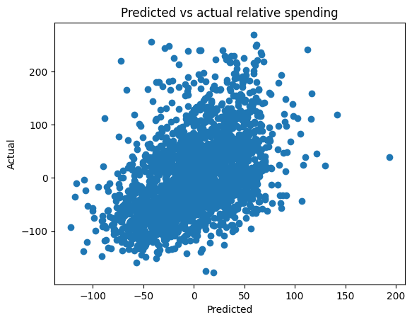
When we look at the predictive power of our best model, we can visually observe the poor correlation. There is, of course, some correlation, and we would expect this - at a very basic level, if the offers were at all effective, I should expect some effect on user spending. However, it is unlikely that we can identify the correct ratios of offers to send to users based on a model with this lack of predictive capability.
I want to revisit our original goal of this model, and to point out why it is not surprising that its predictive power is so poor. This model specifically aims to maximize overall spending from individuals by sending a certain combination of offers, but it fails to do so.
This study, however, has been structured to understand offer success - what types of offers are most likely to be completed by users? I specifically did not use "offer completed" because this is not something that Starbucks directly controls. My model, more simply, asks "Do offers, or certain combinations of offers, result in users who spend more?" At a surface level, my model does not support this hypothesis.
I think this strategy - modeling user spending, as opposed to offer efficacy - could be successful if a longer timer period were available, closer to a year. Anecdotally speaking, I do not see myself going out of my way more than once a month to fulfill an offer from a mobile app. Personally, I am not surprised that a regular user who receives 5 offers in 30 days does not necessarily spend more than a similar user who only received a single offer.
By having a year's worth of data, we could also look at other effects of offers, specifically with "regular customers." As indicated above, the profit base is very largely driven by high spenders, which includes a high spend-per-transaction amount as well as high frequency of visits. I think the value of an offer might be in keeping a customer regular, or encouraging them to stay regular over a long time. Losing a regular customer is a very costly, and we want to protect the profit base as much as possible.
Overall, I think there is value in some of the findings and strategies in this effort, even if the original goal of maximizing user spending through optimizing a spend model was unsuccessful.
I believe the strategy of maximizing profit, as opposed to just chasing better offers, is the correct strategy. I suspect there are other KPIs that are related to profit-per-user that I cannot access due to the short duration of this experiment. User regularity is a major KPI that I would be interested in pursuing - if user regularity can be hardened through the use of effective promotions, then the goal of promotions should be not just to be successful, but to drive user regularity.
In terms of modeling user spend as a function of promotions being offered,I believe this effort was hurt by the lack of data on the low-end - that is, users who received zero or only a single offer. If this study had taken place over a longer period of time, it would be easier to identify periods where a user received no offers, and we could compare this with offer-heavy periods and understand the efficacy of offers in driving spending.
Over the course of this experiment, overall spending per customer did not seem to be driven by the number and types of offers. However, I think my next step would to be looking at "offer available" periods of time. In other words, for a single user, are they more likely to make a purchase if they have an offer available? I am almost certain that this will prove true, and that I would find greater dependencies on things like offer duration and the the value of the promos.
However, I would still stand by my goal of maximizing profit. Do users who only make purchases when it is during an offer window spend more, overall, than users who ignore offers? Additionally, is the cost of redeemed offers worth it for these users? My current study suggests that these may not be true.
Customer regularity, or "stickiness," is a key KPI that I would like to track. This KPI would be much easier to track with a longer study.